Data Engineering Guide

This is my extensive data engineering resource which has all the big data technologies.

FREE DATA ENGINEERING CERTIFICATIONS :

DE Zoom Camp : Link

How does Oozie work?

1. Oozie runs a service in the Hadoop cluster. Client submits workflow to run, immediately or later.

There are two types of nodes in Oozie

1. Action Node – It represents the task in the workflow like MapReduce job, shell script, pig or hive jobs etc.

2. Control flow Node – It controls the workflow between actions by employing conditional logic. In this, the previous action decides which branch to follow.
   Start , End and Error node fall under this category.
   1. Start - signals the start of workflow job
   2. End - designates end of workflow job
   3. Error - signals error and gives and error message

Sqoop :

• Sqoop imports data from external sources into compatible Hadoop Ecosystem components like HDFS, Hive, HBase etc.

• It also transfers data from Hadoop to other external sources

Major difference between Sqoop and Flume - Flume does not work with structured data but Sqoop can work with structured as well as unstructured data.

How does Sqoop work?

1. Submit Sqoop command

2. At back-end, Sqoop gets divided into a number of sub-tasks. [subtasks are map tasks]

3. Each map task imports a part of data to Hadoop.

4. All map-tasks taken together imports the whole data.

5. Sqoop export works in a similar way as Sqoop import except the process is reversed.

FLUME:

• It is a service which helps to ingest structured and semi-structured data into HDFS.

• Works on principle of distributed processing.

• Aids in collection, aggregation and movement of huge amounts of datasets.

Flume has three components:

1. Source – It accepts the data from the incoming stream and stores the data in the channel

2. Channel – It is a medium of temporary storage between the source of the data and persistent storage of HDFS.

3. Sink – This component collects the data from the channel and writes it permanently to the HDFS.

AMBARI :

• Responsible for provisioning , managing, monitoring and securing Hadoop cluster.

Features of Ambari :

1. Simplified cluster configuration, management and installation.

2. Reduced complexity of configuring and administration of Hadoop cluster security.

3. Ensures cluster is healthy and available for monitoring.

Hadoop Cluster provisioning:

• It gives step by step procedure for installing Hadoop services on the Hadoop cluster.

• It also handles configuration of services across the Hadoop cluster.

Hadoop Cluster Management:

• It provides centralized service for starting, stopping and reconfiguring services on the network of machines.

Hadoop Cluster Monitoring :

• To monitor health and status Ambari provides us dashboard.

• Ambari alert framework alerts the user when the node goes down or has low disk space etc.

APACHE SPARK:

• Apache Spark unifies all kinds of Big Data processing under one umbrella.

• It has built-in libraries for streaming, SQL, machine learning and graph processing.

• Apache Spark is lightning fast.

• It gives good performance for both batch and stream processing.

• It does this with the help of DAG scheduler, query optimizer, and physical execution engine.

• Spark does in-memory calculations.

• This makes Spark faster than Hadoop map-reduce.

APACHE SOLR AND LUCENE:

• Two services which search and index the Hadoop ecosystem.

SOLR FEATURES:

1. Scalable , reliable and fault tolerant.

2. Provides distributed indexing, automated failover and recovery, load-balanced query, centralized configuration.

3. You can query Solr using HTTP GET and receive the result in JSON, binary , CSV.

4. MATCHING CAPABILITIES : Abilities to match phrases

5. NEAR REAL TIME INDEXING

HADOOP ARCHITECTURE IN DETAIL:

KEY HADOOP FEATURES:

1. FAULT TOLERANCE

2. HANDLE LARGE DATASETS

3. SCALABLE

Hadoop has a master-slave architecture.

MASTER NODE:

1. Assign a task to various slaves and manage resources.

2. Master node stores metadata. (stores data about data)

SLAVE NODE:

1. Slave nodes do actual computing.

2. They store real data.

Hadoop Architecture comprises three major layers:

1. HDFS

2. YARN

3. MAP-REDUCE

BLOCK SIZE IN HDFS: 128 MB or 256 MB

REPLICATION MANAGEMENT: makes copies of the blocks and stores them on different data nodes. Default replication factor = 3

RACK AWARENESS:

• HDFS follows rack awareness algorithm to place replicas of the blocks in a distributed fashion.

• Rack awareness provides for low latency and fault tolerance.

• Suppose replication factor is 3. Then the rack awareness algorithm will place the first block on a local rack and keep other blocks on a different rack.

• Does not store more than 2 blocks on the same rack if possible.

MAP TASK :

The map task run in the following phase:

1. Record Reader: transforms the input split into records. Provides the data to the mapper function in key-value pairs.

2. Map - user-defined function which processes key-value pair from record reader.

3. Combiner - localized reducer which groups the data in map phase.

4. Partitioner - pulls the intermediate key-value pairs from the mapper. Splits them into shards , one shard per reducer.

REDUCE TASK:

The various phases in reduce task are as follows:

1. Shuffle and Sort: This steps download the data written by partitioner to the machine where reducer is running.

2. Reduce: The reducer performs the reduce function once per key grouping.

3. Output Format : takes the key-value pair from the reducer and writes it to the file by recordwriter. Final data gets written to HDFS.

YARN:

• Basic principle behind YARN is to separate resource management and job scheduling/monitoring function into separate daemons.

• In YARN, there is one global ResourceManager and per-application Application Master.

• An application can be a single job or a DAG of jobs.

Inside the YARN framework , we have two daemons:

1. Resource Manager: arbitrates resources among all competing applications in the system

2. Node Manager: Monitor the resource usage by the container and report the same to Resource Manager.

3. The Application Master negotiates with Resource Manager and works with Node Manager to execute and monitor the job.

The Resource Manager has two main components:

1. Scheduler:

• Responsible for allocating to various applications.

• This is a pure scheduler as it does not perform tracking of status for the application.

• Does not reschedule the task which fail due to software or hardware errors.

• Allocates the resources based on the requirements of the applications.

2. Applications Manager functions:

• Accepts job submission

• Negotiates the first container for executing Application Master. A container incorporates elements such as CPU, memory, disk and network.

• Restarts the ApplicationMaster container on failure.

3. Applications Master functions:

• Negotiates resource container from Scheduler.

• Tracks the resource container status.

• Monitors the progress of the application.

Features of YARN :

1. Multi-tenancy : allows variety of access engines on the same Hadoop data set.

2. Cluster Utilization : allows for good utilization of clusters by dynamic allocation.

3. Scalability : easily expands and copes up with petabytes of data.

HADOOP ADVANTAGES:

1. Varied Data Sources: Accepts a variety of data, structured or unstructured.

2. Cost-effective: economical as it uses cluster of hardware to store data.

3. Fault tolerant: In event of failure of any node, the data block affected can be recovered

4. Scalable: easy to scale

HADOOP DISADVANTAGES:

1. Issue with Small Files: Hadoop is good for small number of large files but not good for large number of small files

2. Vulnerable by Nature: easily exploited cyber criminals

3. Processing Overhead : Data is read from disk and written to disk which makes the read/write operations very expensive. Hadoop cannot do in-memory calculation.

4. Supports Batch Processing.

TEN MOST FREQUENTLY USED HADOOP COMMANDS:

1. Version - shows version of hadoop installed.

2. Mkdir - create directory.

3. Ls - displays contents of the directory.

4. Put - copies the file in the local system to the file in DFS.

5. copyFrom Local : source should refer to local file.

6. Get - copies the file in HDFS to file in local system

7. copyTo Local - similar to get command. Only difference is the destination of copied file should refer to local file.

8. Cat : displays contents of the file on console ot stdout.

9. Mv : moves file from specified source to destination within HDFS.

10. Cp - copies the file from given source to destination within HDFS.

GETMERGE command:

• The getmerge command in Hadoop is for merging files existing in the HDFS file system into a single file in the local file system.

• The command is useful to download the output of MapReduce job. It has multiple part-* files into a single local file.

Three Easy Steps to Execute Hadoop copyFromLocal Command:

Hadoop copyFromLocal:

• We use this command to copy from the local file system to Hadoop Distributed File System

• One Restriction - The source file can only reside in the local file system.

Steps to executes copyFromLocal Command:

1. Make directory

2. Copying the local file into the directory in HDFS

3. Overwriting the existing file in HDFS

What is Hadoop Cluster ? Learn to Build a Cluster in Hadoop

• A Hadoop cluster is nothing but a group of computers connected together via LAN.

• We use it for storing and processing large datasets.

Master in Hadoop Cluster:

There are two daemons running on master:

1. NameNode: Manages file system namespace, stores metadata.

2. Resource Manager: arbitrates resources among competing nodes, keeps track of all live and dead nodes.

Slaves in Hadoop Cluster:

There are two daemons running on Slave machines:

1. Data Node: Stores business data; does read, write and data processing

2. Node Manager: runs service on the node to check its health and reports the same to Resource Manager.

Functions of the client node:

• To load the data on the Hadoop cluster.

• Tells how to process the data by submitting MapReduce job.

• Collects the output from a specified location.

Single Node Hadoop clusters :

• All processes run on the same machine.

• NameNode and DataNode run on the same machine

Multi Node Hadoop clusters:

• Daemon runs on separate host or machines.

• NameNode runs on master machine and DataNode runs on slave machine.

Communication Protocols used in Hadoop Clusters:

Steps:

1. Client establishes a connection with NameNode using configurable TCP port.

2. Hadoop cluster establishes the connection to the client using client protocol.

3. Data Node talks to NameNode using the DataNode protocol.

4. Remote Procedure Call wraps both Client protocol and DataNode protocol.

5. NameNode does not initiate any RPC instead it responds to RPC from the DataNode.

HOW TO BUILD A CLUSTER IN HADOOP:

Before we build a hadoop cluster, we have to understand the following:

1. kind of workloads we will be dealing with

2. Volume of data which cluster need to handle

3. Data retention policy

Sizing the Hadoop Cluster:

• For determining the size of Hadoop cluster, we need to look at how much data is at hand.

• Also, examine the daily data generation.

• This helps us decide the requirements of a number of machines and their configurations.

• Should be a balance between performance and cost of the hardware approved

Hadoop Cluster Management:

A good hadoop cluster management tool should have the following:

• Provide diverse work-load management, security , resource provisioning, performance optimization, health monitoring.

• Implement NameNode high availability with load balancing, auto-failover and hot standby.

• Enabling policy-based controls that prevent any application from gulping more resource than others.

Benefits of Hadoop Clusters:

1. Robustness: The main objective of Hadoop is to store data reliably even in the event of failures. Various kinds of failure is NameNode failure, DataNode failure, and network partition. DataNode periodically sends a heartbeat signal to NameNode. In network partition, a set of DataNodes gets disconnected with the NameNode. Thus NameNode does not receive any heartbeat from these DataNodes. It marks these DataNodes as dead. Also, Namenode does not forward any I/O request to them. The replication factor of the blocks stored in these DataNodes falls below their specified value. As a result, NameNode initiates replication of these blocks. In this way, NameNode recovers from the failure.
   
   

2. Data Disk Failures , Hearbeats and Replication :
   NameNode receives a heartbeat from each DataNode. NameNode may fail to receive heartbeat because of certain reasons like network partition. In this case, it marks these nodes as dead. This decreases the replication factor of the data present in the dead nodes. Hence NameNode initiates replication for these blocks thereby making the cluster fault tolerant.
   
   

3. Cluster Rebalancing: HDFS architecture automatically does rebalancing. Suppose free space on a DataNode falls below a specific threshold level, it automatically moves some data to another DataNode
   
   

4. Data Integrity : Hadoop cluster implements checksum on each block of the file. It does so to see if there is any corruption due to buggy software, faults in storage device etc. If it finds the block corrupted it seeks it from another DataNode that has a replica of the block.

Hadoop High Availability - NameNode Automatic Failover

What is Hadoop High Availability?

Basically, it means that if the NameNode is down , then the system does not stop. It will pass on to the standby node. High Availability overcomes single point of failover in case of routine system maintenance.

What is a failover?

Failover is a process in which the system transfers control to a secondary system in an event of failure.

There are two types of failover:

1. Graceful Failover: The administrator automatically initiates it. We use graceful failover in case of routine system maintenance.

2. Automatic Failover: In Automatic Failover, the system automatically transfers the control to standby NameNode without manual intervention. Acts as insurance against Single Point of Failure.

NameNode High Availability in Hadoop:

Automatic failover in Hadoop adds up below components to a Hadoop HDFS deployment.

Zookeeper Quorum:

• A centralized service for maintaining small amounts of data for coordination, configuration and naming.

• Provides group service and synchronization.

• It keeps the client informed about changes in data and track client failures. Implementation of automatic HDFS failover relies on Zookeeper for:

• Failure detection- Zookeeper maintains a session with NameNode. In the event of failure, this session expires and the zookeeper informs the other NameNodes to start the failover process.

• Active NameNode election- Zookeeper provides a method to elect a node as an active node. Hence whenever his active NameNode fails, other NameNode takes on exclusive lock in the Zookeeper, stating that it wants to become the next active NameNode.

ZKFailoverController (ZKFC) :

Health Monitoring – ZKFC periodically pings the active NameNode with Health check command and if the NameNode doesn’t respond it in time it will mark it as unhealthy. This may happen because the NameNode might be crashed or frozen.

Zookeeper Session Management – If the local NameNode is healthy it keeps a session open in the Zookeeper. If this local NameNode is active, it holds a special lock znode. If the session expires then this lock will delete automatically.

Zookeeper-based Election – If there is a situation where local NameNode is healthy and ZKFC gets to know that none of the other nodes currently holds the znode lock, the ZKFC itself will try to acquire that lock. If it succeeds in this task then it has won the election and becomes responsible for running a failover. The failover is similar to manual failover; first, the previously active node is fenced if required to do so and then the local node becomes the active node.

HADOOP SCHEDULERS:

• Basically, a general-purpose system which enables high-performance processing of data over a set of distributed nodes is what we call Hadoop scheduler.

• Moreover, it is a multitasking system which processes multiple data sets for multiple jobs for multiple users simultaneously.

Three types of schedulers:

1. Hadoop FIFO scheduler:

2. Hadoop Fair Scheduler

3. Hadoop Capacity Scheduler

Hadoop FIFO scheduler:

• An original Hadoop Job Scheduling Algorithm which was integrated within the JobTracker is the FIFO.

• Basically, as a process, a JobTracker pulled jobs from a work queue, that says oldest job first, this is a Hadoop FIFO scheduling.

• Moreover, this is simpler as well as efficient approach and it had no concept of the priority or size of the job.

Hadoop Fair Scheduler:

• Further, to give every user a fair share of the cluster capacity over time, we use the Fair Scheduler in Hadoop.

• It gets all of the Hadoop Clusters if a single job is running.

• Further, free task slots are given to the jobs in such a way as to give each user a fair share of the cluster, as more jobs are submitted.

• If a pool has not received its fair share for a certain period of time, then the Hadoop Fair Scheduler supports preemption.

• Further, the scheduler will kill tasks in pools running over capacity to give the slots to the pool running under capacity.

Hadoop Capacity Scheduler :

• Except for one fact that within each queue, jobs are scheduled using FIFO scheduling in Hadoop (with priorities), this is like the Fair Scheduler.

• It takes a slightly different approach for multiuser scheduling. Moreover, for each user or an organization, it permits to simulate a separate MapReduce Cluster along with FIFO scheduling.

When to use Scheduler?

• The capacity scheduler is the right choice while we want to ensure guaranteed access with the potential in order to reuse unused capacity as well as prioritize jobs within queues, while we are running a large Hadoop cluster, along with the multiple clients.

• Whereas, when we use both small and large clusters for the same organization with a limited number of workloads, the fair scheduler works well.

• Also, in a simpler and less configurable way, it offers the means to non-uniformly distribute capacity to pools (of jobs).

• Furthermore, it can offer fast response times for small jobs mixed with larger jobs (supporting more interactive use models). Hence, it is useful in the presence of diverse jobs.

Distributed Cache:

• Distributed Cache is a facility provided by the Hadoop MapReduce framework.

• It caches files when needed by the applications. It can cache read only text files, archives, jar files etc. Once we have cached a file for our job, Hadoop will make it available on each data nodes where map/reduce tasks are running.

Size of Distributed cache in Hadoop - Default size is 10 GB

Benefits of Distributed Cache in Hadoop :

1. Store Complex Data : distributes simple, read-only text file and complex types like jars, archives

2. Data Consistency: Hadoop Distributed Cache tracks the modification timestamps of cache files. And it notifies that the files should not change until a job is executing. Using hashing algorithm, the cache engine can always determine on which node a particular key-value pair resides. Since, there is always a single state of the cache cluster, it is never inconsistent.

3. Single Point of Failure : A distributed cache runs as an independent process across many nodes. Thus, failure of a single node does not result in a complete failure of the cache.

Hadoop NameNode Automatic Failover:

What is failover?

Failover is the process in which system transfers its control to the secondary system when it detects a fault or failure.

There are two types of Failover:

• Graceful Failover- Administrator manually initiates Graceful Failover, for example, in the case of routine maintenance. The system will not trigger a failover automatically from the active to standby namenode, even if the active node has failed in Graceful Failover.

• Automatic Failover- In the case of NameNode failure, Failover will start automatically. This failover is known as Automatic failover.

LIMITATIONS OF HADOOP :

1. Issue with Small Files

2. Slow Processing Speed

3. Support for Batch Processing Only

4. No Real time Data Processing

SPARK TUTORIAL:

• Spark Programming is nothing but a general-purpose and lightning fast cluster computing platform.

• In other words, it is an open source, wide range data processing engine.

• Spark can perform both batch processing as well as stream processing,

• Spark can access any Hadoop data source and also can run on Hadoop clusters.

• However, Spark is independent of Hadoop since it has its own cluster management system.

• KEY FEATURE - in-memory cluster computation capability

WHY SPARK?

Due to the need of a powerful engine which can respond in sub-second and in-memory processing.

RESILIENT DISTRIBUTED DATASET - RDD

• It is the fundamental unit of data in Spark.

• Immutable in nature.

WAYS TO CREATE SPARK RDD:

1. Parallelize collections: By invoking parallelize method in driver program, we can create parallelized collections.

2. External Datasets: Create Spark RDDs, by calling a textFile method. Hence, this method takes URL of the file and reads it as a collection of lines.

3. Existing RDDs : Moreover, we can create RDDs in spark, by applying transformation operation on existing RDDs.

Spark RDDs operation:

1. Transformation Operation : creates a new RDD from existing one. Moreover, it passes dataset to the function and returns the new dataset.

2. Action Operations: Action returns the final result to the driver program or write it to the external data store.

SPECIAL FEATURES OF RDD:

1. In-memory computation: Basically, while storing data in RDD, data is stored in memory for as long as you want to store. It improves the performance by an order of magnitudes by keeping the data in memory.

2. Lazy Evaluation : Spark Lazy Evaluation means the data inside RDDs are not evaluated on the go. Basically, only after an action triggers all the changes or the computation is performed. Therefore, it limits how much work it has to do.

3. Fault Tolerance : If any worker node fails, by using lineage of operations, we can re-compute the lost partition of RDD from the original one. Hence, it is possible to recover lost data easily

4. Persistence : In in-memory, we can store the frequently used RDD. Also, we can retrieve them directly from memory without going to disk. It results in the speed of the execution. Moreover, we can perform multiple operations on the same data. It is only possible by storing the data explicitly in memory by calling persist() or cache() function.

5. Partitioning : Basically, RDD partition the records logically. Also, distributes the data across various nodes in the cluster. Moreover, the logical divisions are only for processing and internally it has no division. Hence, it provides parallelism.

6. Location-Stickiness : To compute partitions, RDDs are capable of defining placement preference. Moreover, placement preference refers to information about the location of RDD. Although, the DAG Scheduler places the partitions in such a way that task is close to data as much as possible. Moreover, it speeds up computation.

SPARK CONTEXT :

• The most important step of any Spark driver application is to generate SparkContext.

• It allows your Spark Application to access Spark Cluster with the help of Resource Manager (YARN/Mesos).

SPARK STAGE - EXECUTION PLAN

• A stage is nothing but a step in a physical execution plan.

• It is basically a physical unit of the execution plan

• It is a set of parallel tasks i.e. one task per partition.

• In other words, each job which gets divided into smaller sets of tasks is a stage.

• Although, it totally depends on each other.

• However, we can say it is as same as the map and reduce stages in MapReduce.

Two types of Stages:

1. Shuffle Mapstage

2. ResultStage

Types of Spark Stages:

ShuffleMapStage in Spark :

ShuffleMapStage is considered as an intermediate Spark stage in the physical execution of DAG. It produces data for another stage(s). In a job in Adaptive Query Planning / Adaptive Scheduling, we can consider it as the final stage in Apache Spark and it is possible to submit it independently as a Spark job for Adaptive Query Planning.

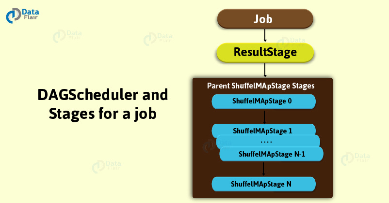
ResultStage in Spark :

By running a function on a spark RDD Stage that executes a Spark action in a user program is a ResultStage. It is considered as the final stage in spark. ResultStage implies as a final stage in a job that applies a function on one or many partitions of the target RDD in Spark. It also helps for computation of the result of an action.

Spark Executor:

Basically, we can say Executors in Spark are worker nodes. Those help to process in charge of running individual tasks in a given Spark job. Moreover, we launch them at the start of a Spark application. Then it typically runs for the entire lifetime of an application. As soon as they have run the task, sends results to the driver. Executors also provide in-memory storage for Spark RDDs that are cached by user programs through Block Manager.

What is Apache Spark RDD?

RDD stands for “Resilient Distributed Dataset”. It is the fundamental data structure of Apache Spark. RDD in Apache Spark is an immutable collection of objects which computes on the different node of the cluster.

Decomposing the name RDD:

• Resilient, i.e. fault-tolerant with the help of RDD lineage graph(DAG) and so able to recompute missing or damaged partitions due to node failures.

• Distributed, since Data resides on multiple nodes.

• Dataset represents records of the data you work with. The user can load the data set externally which can be either JSON file, CSV file, text file or database via JDBC with no specific data structure.

What is RDD Persistence and Caching in Spark?

Spark RDD persistence is an optimization technique in which saves the result of RDD evaluation. Using this we save the intermediate result so that we can use it further if required. It reduces the computation overhead.

What are the Limitations of RDD in Apache Spark?

1. No input optimization engine

2. Runtime type safety

3. Degrade when not enough memory

4. Handling structured data

What is DAG in Apache Spark?

DAG a finite direct graph with no directed cycles. There are finitely many vertices and edges, where each edge directed from one vertex to another. It contains a sequence of vertices such that every edge is directed from earlier to later in the sequence. It is a strict generalization of MapReduce model. DAG operations can do better global optimization than other systems like MapReduce. The picture of DAG becomes clear in more complex jobs.

Apache Spark DAG allows the user to dive into the stage and expand on detail on any stage. In the stage view, the details of all RDDs belonging to that stage are expanded. The Scheduler splits the Spark RDD into stages based on various transformation applied. (You can refer this link to learn RDD

Transformations and Actions in detail) Each stage is comprised of tasks, based on the partitions of the RDD, which will perform same computation in parallel. The graph here refers to navigation, and directed and acyclic refers to how it is done.

APACHE KAFKA:

• Apache Kafka is a fast, scalable, fault-tolerant messaging system which enables communication between producers and consumers using message-based topics.

• In simple words, it designs a platform for high-end new generation distributed applications.

Messaging Systems in Kafka

The main task of managing system is to transfer data from one application to another so that the applications can mainly work on data without worrying about sharing it.

There are two types of messaging patterns available:

• Point to point messaging system

• Publish-subscribe messaging system

• Point to Point Messaging System

In this messaging system, messages continue to remain in a queue. More than one consumer can consume the messages in the queue but only one consumer can consume a particular message.

After the consumer reads the message in the queue, the message disappears from that queue.

• Publish-Subscribe Messaging System

In this messaging system, messages continue to remain in a Topic. Contrary to Point to point messaging system, consumers can take more than one topic and consume every message in that topic. Message producers are known as publishers and Kafka consumers are known as subscribers.

KAFKA ARCHITECTURE

1. Kafka Producer API

This Kafka Producer API permits an application to publish a stream of records to one or more Kafka topics.

2. Kafka Consumer API

The Consumer API permits an application to take one or more topics and process the continous flow of records produced to them.

3. Kafka Streams API

The Streams API permits an application to behave as a stream processor, consuming an input stream from one or more topics and generating an output stream to one or more output topics, efficiently modifying the input streams to output streams.

4. Kafka Connector API

The Connector API permits creating and running reusable producers or consumers that enables connection between Kafka topics and existing applications or data systems.

Kafka Components

1. Kafka Topic

A bunch of messages that belong to a particular category is known as a Topic. Data stores in topics. In addition, we can replicate and partition Topics. Here, replicate refers to copies and partition refers to the division. Also, visualize them as logs wherein, Kafka stores messages. However, this ability to replicate and partitioning topics is one of the factors that enable Kafka’s fault tolerance and scalability.

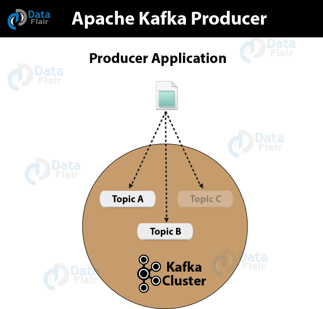
2. Kafka Producer

The producers publish the messages on one or more Kafka topics.

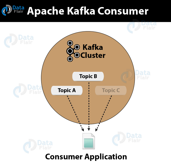
3. Kafka Consumer

Consumers take one or more topics and consume messages that are already published through extracting data from the brokers.

4. Kafka Broker

These are basically systems which maintain the published data. A single broker can have zero or more partitions per topic.

5. Kafka Zookeeper

With the help of zookeeper, Kafka provides the brokers with metadata regarding the processes running in the system and grants health checking and broker leadership election.

Log Anatomy

We view log as the partitions. Basically, a data source writes messages to the log. One of the advantages is, at any time one or more consumers can read from the log they select. Here, the below diagram shows a log is being written by the data source and read by consumers at different offsets.

Data Log

By Kafka, messages are retained for a considerable amount of time. Also, consumers can read as per their convenience. However, if Kafka is configured to keep messages for 24 hours and a consumer is down for greater than 24 hours, the consumer will lose messages. And, messages can be read from last known offset, if the downtime on part of the consumer is just 60 minutes. Kafka doesn’t keep a track on what consumers are reading from a topic.

Partition in Kafka

There are few partitions in every Kafka broker. Each partition can be either a leader or a replica of a topic. In addition, along with updating of replicas with new data, Leader is responsible for all writes and reads to a topic. The replica takes over as the new leader if somehow the leader fails.

KAFKA FEATURES:

a. Scalability

Apache Kafka can handle scalability in all the four dimensions, i.e. event producers, event processors, event consumers and event connectors. In other words, Kafka scales easily without downtime.

b. High-Volume

Kafka can work with the huge volume of data streams, easily.this was all about Apache Kafka Features. Hope you like our explanation.

Kafka offers provision for deriving new data streams using the data streams from producers.

d. Fault Tolerance

The Kafka cluster can handle failures with the masters and databases.

e. Reliability

Since Kafka is distributed, partitioned, replicated and fault tolerant, it is very Reliable.

f. Durability

It is durable because Kafka uses Distributed commit log, that means messages persists on disk as fast as possible.

g. Performance

For both publishing and subscribing messages, Kafka has high throughput. Even if many TB of messages is stored, it maintains stable performance.

h. Zero Downtime

Kafka is very fast and guarantees zero downtime and zero data loss.

i. Extensibility

There are as many ways by which applications can plug in and make use of Kafka. In addition, offers ways by which to write new connectors as needed.

j. Replication

By using ingest pipelines, it can replicate the events.

So, this was all about Apache Kafka Features. Hope you like our explanation.

KAFKA TERMINOLOGIES

i. Kafka Broker

There are one or more servers available in Apache Kafka cluster, basically, these servers (each) are what we call a broker.

ii. Kafka Topics

Basically, Kafka maintains feeds of messages in categories. And, messages are stored as well as published in a category/feed name that is what we call a topic. In addition, all Kafka messages are generally organized into Kafka topics.

iii. Kafka Partitions

In each broker in Kafka, there is some number of partitions. These Kafka partitions in Kafka can be both a leader or a replica of a topic. So, on defining a Leader, it is responsible for all writes and reads to a topic whereas if somehow the leader fails, replica takes over as the new leader.

iv. Kafka Producers

In simple words, the processes which publish messages to Kafka is what we call Producers. In addition, it publishes data on the topics of their choice.

v. Kafka Consumers

The processes that subscribe to topics and process as well as read the feed of published messages, is what we call Consumers.

vi. Offset in Kafka

The position of the consumer in the log and which is retained on a per-consumer basis is what we call Offset. Moreover, we can say it is the only metadata retained on a per-consumer basis.

vii. Kafka Consumer Group

Basically, a consumer abstraction offered by Kafka which generalizes both traditional messaging models of queuing and also publish-subscribe is what we call the consumer group. However, with a consumer group name, Consumers can label themselves.

viii. Kafka Log Anatomy

A log is nothing different but another way to view a partition. Basically, a data source writes messages to the log. Further, one or more consumers read that data from the log at any time they want. Let’s understand it with a diagram, here consumers A and B are reading a data source which is writing to the log and from the log at different offsets.

KAFKA PROS:

a. High-throughput
Without having not so large hardware, Kafka is capable of handling high-velocity and high-volume data. Also, able to support message throughput of thousands of messages per second.

b. Low Latency

It is capable of handling these messages with the very low latency of the range of milliseconds, demanded by most of the new use cases.

c. Fault-Tolerant

One of the best advantages is Fault Tolerance. There is an inherent capability in Kafka, to be resistant to node/machine failure within a cluster.

d. Durability

Here, durability refers to the persistence of data/messages on disk. Also, messages replication is one of the reasons behind durability, hence messages are never lost.

e. Scalability

Without incurring any downtime on the fly by adding additional nodes, Kafka can be scaled-out. Moreover, inside the Kafka cluster, the message handling is fully transparent and these are seamless.

f. Distributed

The distributed architecture of Kafka makes it scalable using capabilities like replication and partitioning.

g. Message Broker Capabilities

Kafka tends to work very well as a replacement for a more traditional message broker. Here, a message broker refers to an intermediary program, which translates messages from the formal messaging protocol of the publisher to the formal messaging protocol of the receiver.

h. High Concurrency

Kafka is able to handle thousands of messages per second and that too in low latency conditions with high throughput. In addition, it permits the reading and writing of messages into it at high concurrency.

i. By Default Persistent

As we discussed above that the messages are persistent, that makes it durable and reliable.

j. Consumer Friendly

It is possible to integrate with the variety of consumers using Kafka. The best part of Kafka is, it can behave or act differently according to the consumer, that it integrates with because each customer has a different ability to handle these messages, coming out of Kafka. Moreover, Kafka can integrate well with a variety of consumers written in a variety of languages.

k. Batch Handling Capable (ETL like functionality)

Kafka could also be employed for batch-like use cases and can also do the work of a traditional ETL, due to its capability of persists messages.

DISADVANTAGES OF KAFKA:

a. No Complete Set of Monitoring Tools

It is seen that it lacks a full set of management and monitoring tools. Hence, enterprise support staff felt anxious or fearful about choosing Kafka and supporting it in the long run.

b. Issues with Message Tweaking

As we know, the broker uses certain system calls to deliver messages to the consumer. However, Kafka’s performance reduces significantly if the message needs some tweaking. So, it can perform quite well if the message is unchanged because it uses the capabilities of the system.

c. Not support wildcard topic selection

There is an issue that Kafka only matches the exact topic name, that means it does not support wildcard topic selection. Because that makes it incapable of addressing certain use cases.

d. Lack of Pace

There can be a problem because of the lack of pace, while API’s which are needed by other languages are maintained by different individuals and corporates.

e. Reduces Performance

In general, there are no issues with the individual message size. However, the brokers and consumers start compressing these messages as the size increases. Due to this, when decompressed, the node memory gets slowly used. Also, compress happens when the data flow in the pipeline. It affects throughput and also performance.

f. Behaves Clumsy

Sometimes, it starts behaving a bit clumsy and slow, when the number of queues in a Kafka cluster increases.

g. Lacks some Messaging Paradigms

Some of the messaging paradigms are missing in Kafka like request/reply, point-to-point queues and so on. Not always but for certain use cases, it sounds problematic.

Applications:

1. Kafka Metrics : For operational monitoring data, Kafka is often used. In addition, to produce centralized feeds of operational data, it includes aggregating statistics from distributed applications.

2. Website Activity Tracking : To be able to rebuild a user activity tracking pipeline as a set of real-time publish-subscribe feeds, it is the original Use Case for Kafka. That implies site activity is published to central topics with one topic per activity type. Here, site activity refers to page views, searches or other actions.

KAFKA ARCHITECTURE:

a. Producer API

In order to publish a stream of records to one or more Kafka topics, the Producer API allows an application.

b. Consumer API

This API permits an application to subscribe to one or more topics and also to process the stream of records produced to them.

c. Streams API

Moreover, to act as a stream processor, consuming an input stream from one or more topics and producing an output stream to one or more output topics, effectively transforming the input streams to output streams, the streams API permits an application.

d. Connector API

While it comes to building and running reusable producers or consumers that connect Kafka topics to existing applications or data systems, we use the Connector API. For example, a connector to a relational database might capture every change to a table.

KAFKA ARCHITECTURE :

a. Kafka Broker

Basically, to maintain load balance Kafka cluster typically consists of multiple brokers. However, these are stateless, hence for maintaining the cluster state they use ZooKeeper. Although, one Kafka Broker instance can handle hundreds of thousands of reads and writes per second. Whereas, without performance impact, each broker can handle TB of messages. In addition, make sure ZooKeeper performs Kafka broker leader election.

b. Kafka – ZooKeeper

For the purpose of managing and coordinating, Kafka broker uses ZooKeeper. Also, uses it to notify producer and consumer about the presence of any new broker in the Kafka system or failure of the broker in the Kafka system. As soon as Zookeeper send the notification regarding presence or failure of the broker then producer and consumer, take the decision and starts coordinating their task with some other broker.

c. Kafka Producers

Further, Producers in Kafka push data to brokers. Also, all the producers search it and automatically sends a message to that new broker, exactly when the new broker starts. However, keep in mind that the Kafka producer sends messages as fast as the broker can handle, it doesn’t wait for acknowledgments from the broker.

d. Kafka Consumers

Basically, by using partition offset the Kafka Consumer maintains that how many messages have been consumed because Kafka brokers are stateless. Moreover, you can assure that the consumer has consumed all prior messages once the consumer acknowledges a particular message offset. Also, in order to have a buffer of bytes ready to consume, the consumer issues an asynchronous pull request to the broker. Then simply by supplying an offset value, consumers can rewind or skip to any point in a partition. In addition, ZooKeeper notifies Consumer offset value.

a. Kafka Topics

The topic is a logical channel to which producers publish message and from which the consumers receive messages.

1. A topic defines the stream of a particular type/classification of data, in Kafka.

2. Moreover, here messages are structured or organized. A particular type of messages is published on a particular topic.

3. Basically, at first, a producer writes its messages to the topics. Then consumers read those messages from topics.

4. In a Kafka cluster, a topic is identified by its name and must be unique.

5. There can be any number of topics, there is no limitation.

6. We can not change or update data, as soon as it gets published.

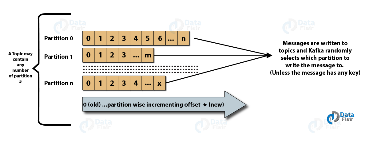
b. Partitions in Kafka

In a Kafka cluster, Topics are split into Partitions and also replicated across brokers.

1. However, to which partition a published message will be written, there is no guarantee about that.

2. Also, we can add a key to a message. Basically, we will get ensured that all these messages (with the same key) will end up in the same partition if a producer publishes a message with a key. Due to this feature, Kafka offers message sequencing guarantee. Though, unless a key is added to it, data is written to partitions randomly.

3. Moreover, in one partition, messages are stored in the sequenced fashion.

4. In a partition, each message is assigned an incremental id, also called offset.

5. However, only within the partition, these offsets are meaningful. Moreover, in a topic, it does not have any value across partitions.

6. There can be any number of Partitions, there is no limitation.

c. Topic Replication Factor in Kafka

While designing a Kafka system, it’s always a wise decision to factor in topic replication. As a result, its topics’ replicas from another broker can solve the crisis, if a broker goes down. For example, we have 3 brokers and 3 topics. Broker1 has Topic 1 and Partition 0, its replica is in Broker2, so on and so forth. It has got a replication factor of 2; it means it will have one additional copy other than the primary one. Below is the image of Topic Replication Factor:

Consumer Group

1. It can have multiple consumer process/instance running.

2. Basically, one consumer group will have one unique group-id.

3. Moreover, exactly one consumer instance reads the data from one partition in one consumer group, at the time of reading.

4. Since, there is more than one consumer group, in that case, one instance from each of these groups can read from one single partition.

5. However, there will be some inactive consumers, if the number of consumers exceeds the number of partitions. Let’s understand it with an example if there are 8 consumers and 6 partitions in a single consumer group, that means there will be 2 inactive consumers.

3. Workflow of Pub-Sub Messaging

In Apache Kafka, the stepwise workflow of the Pub-Sub Messaging is:

• At regular intervals, Kafka Producers send the message to a topic.

• Kafka Brokers stores all messages in the partitions configured for that particular topic, ensuring equal distribution of messages between partitions. For example, Kafka will store one message in the first partition and the second message in the second partition if the producer sends two messages and there are two partitions.

• Moreover, Kafka Consumer subscribes to a specific topic.

• Once the consumer subscribes to a topic, Kafka offers the current offset of the topic to the consumer and save the offset in the Zookeeper ensemble.

• Also, the consumer will request the Kafka in a regular interval, for new messages (like 100 Ms).

• Kafka will forward the messages to the consumers as soon as received from producers.

• The consumer will receive the message and process it.

• Then Kafka broker receives an acknowledgment of the message processed.

• Further, the offset is changed and updated to the new value as soon as Kafka receives an acknowledgment. Even during server outrages, the consumer can read the next message correctly, because ZooKeeper maintains the offsets.

• However, until the consumer stops the request, the flow repeats.

• As a benefit, the consumer can rewind/skip any offset of a topic at any time and also can read all the subsequent messages, as a par desire.

4. Workflow of Kafka Queue Messaging/Consumer Group

A group of Kafka consumers having the same Group ID can subscribe to a topic, instead of a single consumer, in a queue messaging system. However, with the same Group ID all consumers, those are subscribing to a topic are considered as a single group and share the messages. This system’s workflow is:

• In regular intervals, Kafka Producers send the message to a Kafka topic.

• As similar to the earlier scenario, here also Kafka stores all messages in the partitions configured for that particular topic.

• Moreover, a single consumer in Kafka subscribes to a specific topic.

• In the same way as Pub-Sub Messaging, Kafka interacts with the consumer until new consumer subscribes to the same topic.

• As the new customers arrive, share mode starts in the operations and shares the data between two Kafka consumers. Moreover, until the number of Kafka consumers equals the number of partitions configured for that particular topic, the sharing repeats.

• Although, the new consumer in Kafka will not receive any further message, once the number of Kafka consumers exceeds the number of partitions. It happens until any one of the existing consumer unsubscribes. This scenario arises because in Kafka there is a condition that each Kafka consumer will have a minimum of one partition and if no partition remains blank, then new consumers will have to wait.

• In addition, we also call it Kafka Consumer Group. Hence, Apache Kafka will offer the best of both the systems in a very simple and efficient manner.

5. Role of ZooKeeper in Apache Kafka

Apache Zookeeper serves as the coordination interface between the Kafka brokers and consumers. Also, we can say it is a distributed configuration and synchronization service. Basically, ZooKeeper cluster shares the information with the Kafka servers. Moreover, Kafka stores basic metadata information in ZooKeeper Kafka, such as topics, brokers, consumer offsets (queue readers) and so on.

In addition, failure of Kafka Zookeeper/broker does not affect the Kafka cluster. It is because the critical information which is stored in the ZooKeeper is replicated across its ensembles. Then Kafka restores the state as ZooKeeper restarts, leading to zero downtime for Kafka. However, Zookeeper also performs leader election between the Kafka brokers, in the cases of leadership failure.

Hence, this was all about Apache Kafka Workflow.

1. What is Kafka Producer?

Basically, an application that is the source of the data stream is what we call a producer. In order to generate tokens or messages and further publish it to one or more topics in the Kafka cluster, we use Apache Kafka Producer. Also, the Producer API from Kafka helps to pack the message or token and deliver it to Kafka Server.

2. KafkaProducer API

However, to publish a stream of records to one or more Kafka topics, this Kafka Producer API permits to an application. Moreover, its central part is KafkaProducer class. Basically, with the following methods, this class offers an option to connect a Kafka broker in its constructor:

2. What is Kafka Consumer?

An application that reads data from Kafka Topics is what we call a Consumer. Basically, Kafka Consumer subscribes to one or more topics in the Kafka cluster then further feeds on tokens or messages from the Kafka Topics.

What is Kafka Broker?

A Kafka broker is also known as Kafka server and a Kafka node. These all names are its synonyms. In simple words, a broker is a mediator between two. However, Kafka broker is more precisely described as a Message Broker which is responsible for mediating the conversation between different computer systems, guaranteeing delivery of the message to the correct parties.

Hence, the Kafka cluster typically consists of multiple brokers. Kafka Cluster uses Zookeeper for maintaining the cluster state. A single Broker can handle thousands of reads and writes per second. Whereas, if there is no performance impact, each broker can handle TB of messages. In addition, to be very sure that ZooKeeper performs broker leader election.

What is Kafka Connect?

We use Apache Kafka Connect for streaming data between Apache Kafka and other systems, scalably as well as reliably. Moreover, connect makes it very simple to quickly define Kafka connectors that move large collections of data into and out of Kafka.

Kafka Connect collects metrics or takes the entire database from application servers into Kafka Topic. It can make available data with low latency for Stream processing.

a. A common framework for Kafka connectors

It standardizes the integration of other data systems with Kafka. Also, simplifies connector development, deployment, and management.

b. Distributed and standalone modes

Scale up to a large, centrally managed service supporting an entire organization or scale down to development, testing, and small production deployments.

c. REST interface

By an easy to use REST API, we can submit and manage connectors to our Kafka Connect cluster.

d. Automatic offset management

However, Kafka Connect can manage the offset commit process automatically even with just a little information from connectors. Hence, connector developers do not need to worry about this error-prone part of connector development.

e. Distributed and scalable by default

It builds upon the existing group management protocol. And to scale up a Kafka Connect cluster we can add more workers.

f. Streaming/batch integration

We can say for bridging streaming and batch data systems, Kafka Connect is an ideal solution.

3. Why Kafka Connect?

As we know, like Flume, there are many tools which are capable of writing to Kafka or reading from Kafka or also can import and export data. So, the question occurs, why do we need Kafka Connect. Hence, here we are listing the primary advantages:

9. Kafka Connector Types

By implementing a specific Java interface, it is possible to create a connector. We have a set of existing connectors, or also a facility that we can write custom ones for us.

Its worker simply expects the implementation for any connector and task classes it executes to be present in its classpath. However, without the benefit of child classloaders, this code is loaded directly into the application, an OSGi framework, or similar.

There are several connectors available in the “Confluent Open Source Edition” download package, they are:

• JDBC

• HDFS

• S3

• Elasticsearch

8. REST API

Basically, each worker instance starts an embedded web server. So, through that, it exposes a REST API for status-queries and configuration. Moreover, configuration uploaded via this REST API is saved in internal Kafka message broker topics, for workers in distributed mode. However, the configuration REST APIs are not relevant, for workers in standalone mode.

By wrapping the worker REST API, the Confluent Control Center provides much of its Kafka-connect-management UI.

To periodically obtain system status, Nagios or REST calls could perform monitoring of Kafka Connect daemons potentially.

3. Tuning Kafka for Optimal Performance

TUNING KAFKA PRODUCERS:

i. Batch Size

Instead of the number of messages, batch.size measures batch size in total bytes. That means it controls how many bytes of data to collect, before sending messages to the Kafka broker. So, without exceeding available memory, set this as high as possible. Make sure the default value is 16384.

ii. Linger Time

In order to buffer data in asynchronous mode, linger.ms sets the maximum time. Let’s understand it with an example, a setting of 100 batches 100ms of messages to send at once. Here, the buffering adds message delivery latency but this improves throughput.

b. Tuning Kafka Brokers

As we know, Topics are divided into partitions. Further, each partition has a leader. Also, with multiple replicas, most partitions are written into leaders. However, if the leaders are not balanced properly, it might be possible that one might be overworked, compared to others.

So, on the basis of our system or how critical our data is, we want to be sure that we have sufficient replication sets to preserve our data. It is recommended that starting with one partition per physical storage disk and one consumer per partition.

c. Tuning Kafka Consumers

Basically, Kafka Consumers can create throughput issues. It is must that the number of consumers for a topic is equal to the number of partitions. Because, to handle all the consumers needed to keep up with the producers, we need enough partitions.

In the same consumer group, consumers split the partitions among them. Hence, adding more consumers to a group can enhance performance, also adding more consumer groups does not affect performance.

What is NoSQL Database?

Before starting MongoDB Tutorial, we must know about NoSQL. NoSQL or “non-SQL” a non-structured database. It provides a facility for storage and retrieval of data using fields. While in SQL the data stores in a tabular form. Companies are using a NoSQL database in big data and real-time applications. NoSQL offers “eventual consistency” so that it may not meet the real-time application requirements. Still, its use to merits over relational databases.

What is MongoDB?

MongoDB is an open source platform written in C++ and has a very easy setup environment. It is a cross-platform, document-oriented and non-structured database. MongoDB provides high performance, high availability, and auto-scaling.

It is a NoSQL database and has flexibility with querying and indexing. MongoDB has very rich query language resulting in high performance.

MongoDB Features

Here, in this part of the MongoDB Tutorial, we discuss some key features of MongoDB:

i. Ad-hoc Queries

MongoDB supports ad-hoc queries by indexing.

ii. Schema-Less Database

It is very flexible than structured databases. There is no need to type mapping.

iii Document Oriented

It is document oriented, JSON like a database.

iv. Indexing

Any document can index with primary and secondary indices.

v. Replication

It has this powerful tool. Every document has one primary node which further has two or more secondary replications.

vi. Aggregation

For efficient usability, MongoDB has aggregation framework for batch processing.

vii. GridFS

It has grid file system, so it can use to store files in multiple machines.

viii. Sharding

For the larger data sets sharding is the best feature. It distributes larger data to multiple machines.

ix. High Performance

Indexes support faster queries leading to high performance.

Ad-hoc Queries

Generally, when we design a schema of a database, we don’t know in advance about the queries we will perform. Ad-hoc queries are the queries not known while structuring the database. So, MongoDB provides ad-hoc query support which makes it so special in this case. Ad-hoc queries are updated in real time, leading to an improvement in performance.

Schema-Less Database

In MongoDB, one collection holds different documents. It has no schema so can have many fields, content, and size different than another document in the same collection. This is why MongoDB shows flexibility in dealing with the databases.

Document-Oriented

MongoDB is a document-oriented database, which is a great feature itself. In the relational databases, there are tables and rows for arrangements of the data. Every row has specific no. of columns & those can store a specific type of data. Here comes the flexibility of NoSQL where there are fields instead of tables and rows. There are different documents which can store different types of data. There are collections of similar documents. Each document has a unique key id or object id which can both be user or system defined.

Indexing

Indexing is very important for improving the performances of search queries. When we continuously perform searches in a document, we should index those fields that match our search criteria. In MongoDB, we can index any field indexed with primary and secondary indices. Making query searches faster, MongoDB indexing enhances the performance.

Replication

When it comes to redundancy, replication is the tool that MongoDB uses. This feature distributes data to multiple machines. It can have primary nodes and their one or more replica sets. Basically, replication makes ready for contingencies. When the primary node is down for some reasons, the secondary node becomes primary for the instance. This saves our time for maintenance and makes operations smooth.

Aggregation

MongoDB has an aggregation framework for efficient usability. We can batch process data and get a single result even after performing different operations on the group data.

The aggregation pipeline, map-reduce function, and single purpose aggregation methods are the three ways to provide an aggregation framework.

GridFS

GridFS is a feature of storing and retrieving files. For files larger than 16 MB this feature is very useful. GridFS divides a document in parts called chunks and stores them in a separate document. These chunks have a default size of 255kB except the last chunk.

When we query GridFS for a file, it assembles all the chunks as needed.

Sharding

Basically, the concept of sharding comes when we need to deal with larger datasets. This huge data can cause some problems when a query comes for them. This feature helps to distribute this problematic data to multiple MongoDB instances.

The collections in the MongoDB which has a larger size are distributed in multiple collections. These collections are called “shards”. Shards are implemented by clusters.

Advantages Of MongoDB

Sharding

We can store a large data by distributing it to several servers connected to the application. If a server cannot handle such a big data then there will be no failure condition. The term we can use here is “auto-sharding”.

Flexible Database

We know that MongoDB is a schema-less database. That means we can have any type of data in a separate document. This thing gives us flexibility and a freedom to store data of different types.

High Speed

MongoDB is a document-oriented database. It is easy to access documents by indexing. Hence, it provides fast query response. The speed of MongoDB is 100 times faster than the relational database.

High Availability

MongoDB has features like replication and gridFS. These features help to increase data availability in MongoDB. Hence the performance is very high.

Scalability

A great advantage of MongoDB is that it is a horizontally scalable database. When you have to handle a large data, you can distribute it to several machines.

Disadvantages Of MongoDB

a. Joins not Supported

MongoDB doesn’t support joins like a relational database. Yet one can use joins functionality by adding by coding it manually. But it may slow execution and affect performance.

b. High Memory Usage

MongoDB stores key names for each value pairs. Also, due to no functionality of joins, there is data redundancy. This results in increasing unnecessary usage of memory.

c. Limited Data Size

You can have document size, not more than 16MB.

d. Limited Nesting

You cannot perform nesting of documents for more than 100 levels.

This was all about Advantages Of MongoDB Tutorial. Hope you like our explanation.

MongoDB Vs RDBMS

Following are some of the points which tell us the difference between MongoDB and RDBMS.

• RDBMS is having a relational database but MongoDB has a non-relational database.

• In RDBMS we need to design the table then only we can start coding but in MongoDB, we can directly start coding.

• RDBMS supports SQL language and MongoDB supports SQL as well as JSON query language.

• RDBMS is table based whereas MongoDB is key-value based.

• MongoDB is document based whereas RDBMS is row based.

• RDBMS is column based whereas MongoDB is field based.

• RDBMS is not that easy to set up but MongoDB is comparatively easy to set up.

• MongoDB is horizontally scalable, on the other hand, RDBMS is vertically scalable.

• RDBMS processes the data very slow as compared to the unstructured data of MongoDB.

• RDBMS accentuates on ACID (Atomicity, Consistency, Isolation, Durability) properties. On the other hand, MongoDB accentuates on CAP (Consistency, Availability, Partition tolerance) theorem.

i. Queries

It supports range query, regular expression and many more types of searches for queries. MongoDB supports ad-hoc and document-based queries. Queries include user-defined JavaScript functions and can also return specific kind of data out of the document. It can also return a random sample of data of a given specified size.

ii. Indexing

Fields in the document can be indexed either as primary or secondary. MongoDB is also capable of handling and dealing with the replication in data. As we know that replica sets contain the same data with more than one copy of itself. Each replica will try to put itself in either the primary or secondary index. Generally all the read and write processing on the data is done by using the primary index but sometimes it may happen that the primary index of the replica fails due to some reason.

So at that time, the replica set goes under election process as to which secondary index of replica should be chosen to go for further processing by either read or write operation. Most of the times the secondary one is being used for a write operation and it is rarely being used for reading operation.

iii. Load Imbalance

With the help of sharding MongoDB scales horizontally. The user is given a chance to choose a shared key with the help of which it can determine, how the data in a collection will be distributed. Here, the data is being split into ranges based on the shard key and then is distributed across multiple shards. Here, the shard will act as a master with one or more slaves with itself. This can also be done with the help of hashing which will result in even distribution of data all along.

iv. Handling multiple servers

MongoDB can run on multiple servers at the same time while handling the duplicate data and also balancing a load of data even in cases, where there might be chances of hardware failure.

v. File storage system

This mechanism of storing the data while handling the load and also checking out for any replication of the same data at multiple sites is called as GridFS (Grid File System). This function is being added with the MongoDB drivers. GridFS can be accessed with the help of mongofiles utility or different kind of plugins. GridFS breaks the file into smaller parts and stores each part as a separate document.

vi. Aggregation

It has three different ways to perform aggregation and they are as follows:

• Aggregation pipeline

• Map-Reduce function

• Single Purpose Aggregation Methods.

In the aggregation pipeline, they use pipelining so that the processor is not an ideal state and also that each process is related to the output of the earlier process in the pipeline.

Map-reduce can be used to do batch processing of data and aggregation operation too. But this can be handled well with the help of aggregation pipeline.

vii. High Performance

Here, the input/output operations take less time to execute as compared to the relational database. Queries are also being executed in a fast pace as compared to the relational database.

What is MongoDB Data Modeling?

• We know that MongoDB is a document-oriented database or NoSQL database.

• It is a schema-less database or we can say, it has a flexible schema.

• Unlike the structured database, where we need to determine table’s schema in advance, MongoDB is very flexible in this area.

• MongoDB deals in collections, documents, and fields.

• We can have documents containing different sets of fields or structures in the same collection.

• Also, common fields in a collection can contain different types of data. This helps in easy mapping.

The key challenge in MongoDB data modeling is balancing the requirements of the application. Also, we need to assure the performance aspect effectively while modeling. Let’s point out some requirements while MongoDB Data Modeling taking place.

1. Design schema according to the need.

2. Objects which are queried together should be contained in one document.

3. Consider the frequent use cases.

4. Do complex aggregation in the schema.

MongoDB Document Structure

There can be two ways to establish relationships between the data in MongoDB:

• Referenced Documents

• Embedded Documents

a. Referenced Documents

Reference is one of the tools that store the relationship between data by including links from one data to another. In such data, a reference to the data of one collection will be used to collect the data between the collections. We can say, applications resolve these references to access the related data. These are normalized data models.

Reference relationships should be used to establish one to many or many to many relationships between documents. Also, when the referenced entities are frequently updated or grow indefinitely.

Embedded Documents

These can be considered as de-normalized data models. As the name suggests, embedded documents create relationships between data by storing related data in a single document structure. These data models allow applications to retrieve and manipulate related data in a single database operation.

Embedded documents should be considered when the embedded entity is an integral part of the document and not updated frequently. It should be used when there is a contained relation between entities and they should not grow indefinitely

Considerations for MongoDB Data Modeling

Some special consideration should give while designing a data model of MongoDB. This is for high per performance scalable and efficient database. The following aspects should consider for MongoDB Data Modeling.

a. Data Usage

While designing a data model, one must consider that how applications will access the database. Also, what will be the pattern of data, such as reading, writing, updating, and deletion of data. Some applications are read centric and some are write-centric. There are possibilities that some data use frequently whereas some data is completely static. We should consider these patterns while designing the schema.

b. Document growth

Some updates increase the size of the documents. During initialization, MongoDB assigns a fixed document size. While using embedded documents, we must analyze if the subobject can grow further out of bounds. Otherwise, there may occur performance degradation when the size of the document crosses its limit. MongoDB relocates the document on disk if the document size exceeds the allocated space for that document.

c. Atomicity

Atomicity in contrast to the database means operations must fail or succeed as a single unit. If a parent transaction has many sub-operations, it will fail even if a single operation fails. Operations in MongoDB happen at the document level. No single write operation can affect more than one collection. Even if it tries to affect multiple collections, these will treat as separate operations. A single write operation can insert or update the data for an entity. Hence, this facilitates atomic write operations.

However, schemas that provide atomicity in write operations may limit the applications to use the data. It may also limit the ways to modify applications. This consideration describes the challenge that comes in a way of data modeling for flexibility.

What is MongoDB Index?

For any kind of database, indexes are of great importance. In MongoDB, Indexes helps to solve queries more efficiently. Indexes are a special data structure used to locate the record in the given table very quickly without being required to traverse through every record in the table. MongoDB uses these indexes to limit the number of documents that had to be searched in a collection. The data structure that is used by an index is a Binary Tree.

Types of Index in MongoDB

Single Field Index

MongoDB supports user-defined indexes like single field index. A single field index is used to create an index on the single field of a document. With single field index, MongoDB can traverse in ascending and descending order. That’s why the index key does not matter in this case.

Compound Index

MongoDB supports a user-defined index on multiple fields as well. For this MongoDB has a compound index. There sequential order of fields for a compound index.

For example, if a compound index consists of {“name”:1,”city”:1}), then the index will sort first the name and then the city.

Multikey Index

MongoDB uses the multikey indexes to index the values stored in arrays. If we index a field with an array value, MongoDB creates separate index entries for each element of the array. These indexes allow queries to select documents with the matching criteria.

MongoDB automatically determines whether to create a multikey index if the indexed field contains an array value. We do not need to specify the multikey type explicitly. Below is the example of a multikey index.

Geospatial Index

To query geospatial data, MongoDB supports two types of indexes – 2d indexes and 2d sphere indexes. 2d indexes use planar geometry when returning results and 2dsphere indexes use spherical geometry to return results.

Text Index

It is another type of index that is supported by MongoDB. Text index supports searching for string content in a collection. These index types do not store language-specific stop words (e.g. “the”, “a”, “or”). Text indexes restrict the words in a collection to only store root words.

What is MongoDB Replication?

As the name says, MongoDB replication means instances that maintain the same data set. It contains several data bearing nodes and optionally one arbiter node. Out of all the data bearing nodes, only one of them is a primary node while the others are secondary nodes. A primary node can do all the write operations. A replica set containing primary node is can confirm writes with {w: “majority”}.

The secondary nodes replicate the primary one and apply the operations to their respective dataset. When the data is reflected in the second one it also changes on the primary dataset. If the primary node is not available then the secondary nodes from themselves can elect one of them as a primary node.

Here arbiters do not have a dataset with themselves. Its purpose is to maintain a quorum in a replica set by responding to heartbeat and election requests by other replica members. If your replica set has an even number of members, add an arbiter to obtain a majority of votes in an election for a primary node.

Automatic Failover

When a primary node does not communicate with other members of the set for a certain period of time i.e. electionTimeoutMills(10 seconds by default) period, then an eligible secondary node calls out for an election. The clusters present over here try to complete the election as fast as possible so that they can return to the normal operations to be performed.

What is MongoDB Sharding?

A sharded cluster consists of the following components:

• shard: They contain the subset of sharded data. Each shard can be deployed as a replica set.

• mongos: They act as a query router. They also provide an interface between client applications and a sharded cluster.

• config server: They store metadata and configuration settings for the cluster. From MongoDB 3.4 onwards config server must be deployed as a replica set (CSRS).

MongoDB Sharding Strategies

There are two types of strategies offers by MongoDB Sharding:

1. Hashed Sharding

2. Ranged Sharding

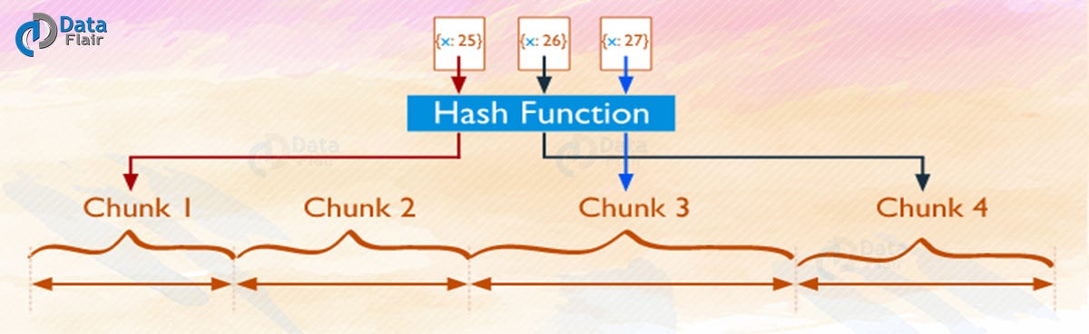
i. Hashed Sharding in MongoDB

It involves computing a hash of the shard key field’s value. Each chunk is assigned a range according to the hash value.

Ranged Sharding in MongoDB

It involves dividing data into ranges based on the shard key values. After that, each chunk is assigned some value based on the shard keys.

A range of shard keys who are having very close values is supposed to be present in the same chunk. Its efficiency depends upon the shard key chosen. In the worst case shard keys can result in uneven distribution of data, which

results in opposition to some benefits of sharding in MongoDB.